How is the Southern Ocean climate represented in ocean-sea ice models forced by the same atmospheric state?

Time-mean and trends for the period 1948-2007 are analysed in a suite of global ocean-sea ice models forced with CORE-II forcing, focusing on the ACC, MOC, water masses and sea-ice evolution.
The second phase of the Coordinated Ocean-ice Reference Experiments (CORE-II), organized by the CLIVAR Ocean Model Development Panel (OMDP), is resulting in several publications focusing on different oceanic regions and processes. Using many different state-of-the-art global ocean-sea ice models forced with the same atmospheric state spanning 1948-2007, CORE-II studies aim to present a comprehensive overview of ocean-sea ice climate model simulations with respect to observations, and theoretical and previous modelling studies. More information can be found here: http://www.clivar.org/clivar-panels/omdp/core-2.
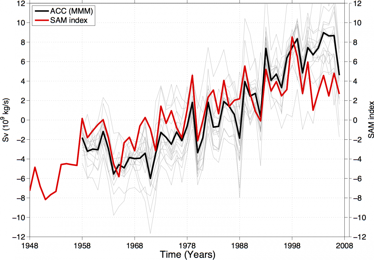
These two papers, recently published in the CORE-II virtual special issue in Ocean Modelling, focus on the Southern Ocean region in models with resolution varying from coarse to eddy-permitting. The first study assesses the representation of the Antarctic Circumpolar Current (ACC) and Meridional Overturning Circulation (MOC) (Farneti et al., 2015). The authors quantify the degree of eddy saturation and eddy compensation in the models, a topic that has sparked the interest of both theoreticians and modellers in the last few years not only in the pursuit of its physical understanding but also because of the fundamental role that the Southern Ocean plays in a warming climate. Given the relatively small wind changes that occurred during the past 50 years, Farneti et al. (2015) show that most models experienced weak ACC transport sensitivity to changes in winds, and they were considered to be in an eddy saturated regime. Larger differences arise when considering changes in the MOC, with a majority of models exhibiting significant strengthening of the MOC. Only eddy-permitting models and models using a parameterization with a three-dimensional time varying coefficient showed some degree of eddy compensation, as well as weaker changes in isopycnal slopes and associated ACC trends. Also, both ACC and MOC interannual variability was largely controlled by the Southern Annular Mode (SAM) in the CORE-II runs (Figure 1).
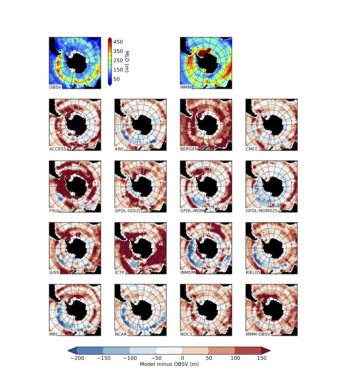
The second study focuses on the representation of water mass properties and sea-ice processes (Downes et al., 2015). Recent multi-model analyses have shown large discrepancies in mixed layer depths and sea-ice trends (for example, models failing to capture increases in sea ice in the Ross Sea). The mixed layer depth is tightly linked to the flux of water masses into the ocean interior. Downes et al. (2015) show the CORE-II state likely influences the current climate summer and winter mixed layer depths and positions (Figure 2), the upper ocean temperature and salinity biases versus observations, and the summer sea ice concentration. However, the individual ocean and ice model density fields and parameterisations (such as overflow processes and mesoscale mixing schemes) dictate the exchange between water masses, and the decadal trends in the winter mixed layers and sea ice. Biases in the CORE-II state (e.g., winds over the Antarctic continent), primarily due to insufficient observations, also contribute to the models’ misrepresentation of recently observed climate trends.
Written by Riccardo Farneti and Stephanie Downes.
Figure 1: The multi-model-mean (MMM) Drake Passage transport anomalies (with respect to the 1958-2007 mean; in Sv) are shown by the black line, gray lines refer to individual models transport anomalies, and the SAM index is shown by the red line (right axis). The MMM-SAM correlation is 0.77.

Figure 2: First two top row panels: observed (de Boyer Montegut et al., 2004, OBSV) and multi-model mean (MMM) September mixed layer depth (m), defined as using a 0.03 kg m-3 criterion. Remaining panels (associated color scale at bottom of figure): individual models and multi model mean (1988-2007 average) minus observations. Note: the color bar in the top row represents the mean states of the observations and multi model mean, whereas the color bar at the bottom of the figure is for the remaining rows (the biases from observations).


